Support:Documents:Examples: Reslicing using COMKAT image tool (advanced)
Estimation of Physiological Parameters Using a Physiologically Based Model
Overview
To evaluate glucose transport and phosphorylation in skeletal muscle, a physiologically based model has been proposed by our group. Herein, we show an example of implementation of the proposed model using COMKAT software. In particular, the below example shows the implementation of the proposed model for a phosphorylatable glucose analog (e.g. 18F-labeled 2-fluoro-2-deoxy-D-glucose).
The above figure shows the kinetics of [18F]2FDG in skeletal muscle. The model has three tissue compartments with five rate constants.
The first compartment is the interstitial concentration of [18F]2FDG .
The second compartment is the intracellular concentration of [18F]2FDG .
The third compartment is the intracellular concentration of [18F]2FDG-6-P .
Rate constants k1 and k2 describe the passive exchange of the glucose analog between plasma and interstitial space.
Rate constants k3a and k4a describe the inward and backward transport of the glucose analog via glucose transporters.
Rate constant k5a describe the phosphorylation of the intracellular glucose analog catalyzed by hexokinase.
COMKAT Implementation of the Physiologically Based Model
Create a new model
cm=compartmentModel;

% Define parameters
cm=addParameter(cm,'k1',0.1);
cm=addParameter(cm,'k2','k1/Fis');
cm=addParameter(cm,'k3','VG/(Fis*KGa+Fis*ISg*KGa/KGg)');
cm=addParameter(cm,'k4','VG/(Fic*KGa+Fic*ICg*KGa/KGg)');
cm=addParameter(cm,'k5','VH/(Fic*KHa+Fic*ICg*KHa/KHg)');

cm=addParameter(cm,'Fb',0.02);         % fraction of total space occupied by blood
cm=addParameter(cm,'Fis',0.3);          % fraction of total space occupied by interstitial space
cm=addParameter(cm,'Fic','1-Fis-Fb');  % fraction of total space occupied by intracellular space

cm=addParameter(cm,'Pg',6);     % Plasma glucose concentration (mM)
cm=addParameter(cm,'ISg',5.4); % Interstitial glucose concentration (mM)
cm=addParameter(cm,'ICg',0.2); % Intracellular glucose concentration (mM)

cm=addParameter(cm,'KGg',3.5); % Michaelis constant (mM) of glucose transporter (GLUT) for glucose
cm=addParameter(cm,'KHg',0.13); % Michaelis constant (mM) of hexokinase (HK) for glucose

cm=addParameter(cm,'KGa',14); % Michaelis constant (mM) of GLUT for glucose analog
cm=addParameter(cm,'KHa',0.17); % Michaelis constant (mM) of HK for glucose analog

cm=addParameter(cm,'VG','(k1*Pg-k1*ISg)/(ISg/(KGg+ISg)-ICg/(KGg+ICg))'); % Maximal velocity of glucose transport for glucose and its analogs
cm=addParameter(cm,'VH','(k1*Pg-k1*ISg)/(ICg/(KHg+ICg))'); % Maximal velocity of glucose phosphorylation for glucose and its analogs

% Define compartment
cm=addCompartment(cm,'IS'); % interstitial
cm=addCompartment(cm,'IC'); % intracellular
cm=addCompartment(cm,'IP'); % intracellular phosphorylated
cm=addCompartment(cm,'Junk');

% Define link
cm=addLink(cm,'L','Cp','IS','k1');
cm=addLink(cm,'K','IS','Junk','k2');
cm=addLink(cm,'K','IS','IC','k3');
cm=addLink(cm,'K','IC','IS','k4');
cm=addLink(cm,'K','IC','IP','k5');
Specify the input, output and scan time
% Specific activity (sa): if the unit of image data is the same with that of input function, the specific activity is 1.
cm=addParameter(cm,'sa',1);
% Usually, the decay time correction of image data is performed. So, dk is zero.
cm=addParameter(cm,'dk',0);

% Define scan time (minutes)
delay = 0.0;
scanduration = 120;

t=[ones(5,1)/30;ones(10,1)/12;ones(12,1)*0.5;ones(8,1);ones(21,1)*5];
scant = [[0;cumsum(t(1:(length(t)-1)))] cumsum(t)];
scanTime  = [scant(:,1),scant(:,2)];

cm = set(cm, 'ScanTime', scanTime);

lambda = [-12.02 -2.57 -0.02];

a = [1771.5 94.55 14.27];

cm = addParameter(cm, 'pfeng', [delay a lambda]');

% Define input function
cm = addInput(cm, 'Cp', 'sa', 'dk', 'fengInputByPar','pfeng'); % Cp is the plasma input function
cm = addInput(cm, 'Ca',1,0, 'fengInputByPar', 'pfeng'); % Ca is the decay-corrected whole-blood input function. Herein, we assume that Cp=Ca.

% Define output obtained from each normalized compartment
wlistTotal={'IS',1;'IC',1;'IP',1};
xlistTotal={'Ca','Fb'};
cm=addOutput(cm,'TissueTotal',wlistTotal,xlistTotal);
Usually, the model outputs consist of compartments and weights with which they contribut to outputs (e.g. Fis*IS, Fic*IC, Fic*IP).
However, as described in detail in our published paper, tracer concentrations of all compartments (i.e. IS, IC and IP) in final model equations are normalized to total tissue space.
Accordingly, the weights of these compartment are 1.
Solve the model output and Generate synthetic data
[PET,PETIndex,Output,OutputIndex]=solve(cm);

noise_level=0.05;

sd=noise_level*sqrt(PET(:,3)./(PET(:,2)-PET(:,1)));

data=sd.*randn(size(PET(:,3)))+PET(:,3);

cm=set(cm,'ExperimentalData',data);

cm = set(cm,'ExperimentalDataSD',sd);

figure;
t = 0.5*(PET(:,1)+PET(:,2));
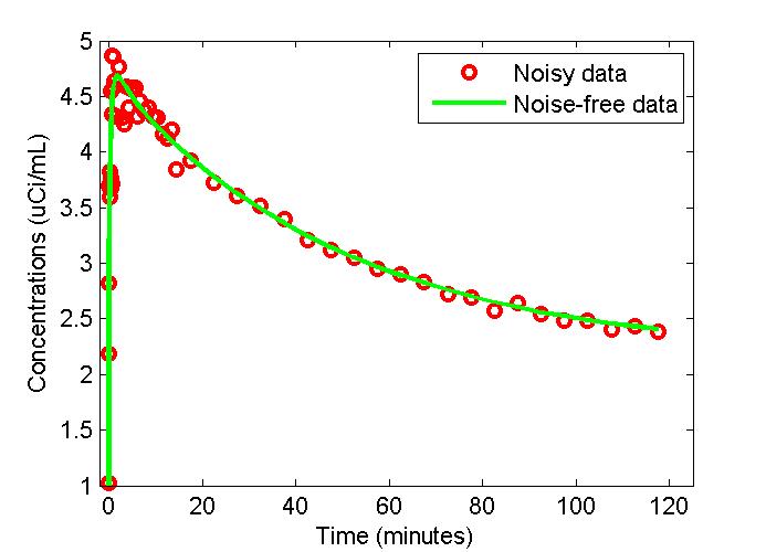
plot(t,PET(:,3),'g-',t,data,'ro','LineWidth',2);
xlabel('Time (minutes)');
ylabel('Concentrations (uCi/mL)');
legend('Noisy data','Noise-free data');
Fit Data
% Define model parameters to be estimated
cm=addSensitivity(cm,'k1','ISg','ICg','Fis','Fb');

optsIRLS = setopt('SDModelFunction', @IRLSnoiseModel);
cm = set(cm, 'IRLSOptions', optsIRLS);

oo = optimset('TolFun', 1e-8, 'TolX', 1e-4,'Algorithm','interior-point');
cm = set(cm, 'OptimizerOptions', oo);

% Set initial conditions and bounds
%        k1,    ISg,   ICg,     Fs,     Fb
pinit = [0.01  ; 4.4 ; 0.1    ;0.15 ; 0.01];
plb   = [0.001; 1    ; 0.001;0.10 ; 0     ];
pub  = [0.5   ; 6    ; 1       ;0.60 ; 0.04];

[pfit, qfit, modelfit, exitflag, output, lambda, grad, hessian, objfunval] = fitGen(cm, pinit, plb, pub, 'IRLS');
Results
figure;
t = 0.5*(PET(:,1)+PET(:,2));
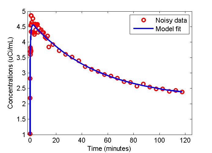
plot(t,data,'ro',t,modelfit,'b-','LineWidth',2);
xlabel('Time (minutes)');
ylabel('Concentrations (uCi/mL)');
legend('Noisy data', 'Model fit');

Pg=6;KGa=14;KHa=0.17;KGg=3.5;KHg=0.13; % Units are mM

k1=pfit(1);k2=pfit(1)/pfit(4);ISg=pfit(2);ICg=pfit(3);Fis=pfit(4);Fb=pfit(5);

% Physiological parameters

VG=(k1*Pg-k1*ISg)/(ISg/(KGg+ISg)-ICg/(KGg+ICg))

VH=(k1*Pg-k1*ISg)/(ICg/(KHg+ICg))

CI=VG*ISg/(KGg+ISg)

CE=VG*ICg/(KGg+ICg)

PR=VH*ICg/(KHg+ICg)


