Support:Documents:Examples:Estimate Input Delay and Rate Constants
Estimating Input Delay and Rate Constants
This example demonstrates an approach to simultaneously estimating input function delay along with parameters of the 1-tissue compartment (e.g. blood flow) model. For the sake of generality, this could be interpreted as a dynamic contrast-enhanced (DCE) MRI or perfusion PET study.
Tissue uptake
This model has one tissue compartment. Material in the blood is assumed to rapidly exchange with that in (extravascular) tissue. The tissue model has two rate constants: K1 and k2 and is depicted in the diagram:
It can also be described by the differential equation:
dCT/dt = K1 Cp - k2 CT
where CT is the tissue concentration and Cp is the plasma concentration.
CT and Cp are interpreted as either molar concentrations (Salinas, Muzic and Saidel 2007).
Input function
This example also demonstrates how to temporally align measured input function data to the tissue (image) data. Here the plasma concentration vs. time t is modeled as
Cp(t, tau) = M(t-tau) if t >= tau; 0 if t < tau .
M(t) is the measured input data, tau is the delay parameter to estimate, and t is the time in minutes.
Because the delay tau is estimated in this example, it will be handy to note that derivative of the input with respect to delay is
dCp(t)/d tau = - dM/dt|t-tau
For this example, M is determined by using linear interpolation to interpolate between measured values. The interpolation is implemented using piecewise polynomial framework (and it could be easily modified to accommodate cubic spline interpolation).
Let inputData be a two-column matrix with column 1 holding sample times and column 2 holding the sampled input concentrations.
The interpolation coefficients may be calculated using the lspline function
ppM = lspline(inputData(:,1), inputData(:,2));
To evaluate the derivative dCp/dt, which can be determined in terms of dM/dt by analytically differentiating the interpolating polynomial.
[breaks, coefs, l, k, d] = unmkpp(ppM);
ppdMdtau = mkpp(breaks, repmat(k-1:-1:1,d*l,1) .* coefs(:,1:k-1), d);
The input function is then implemented as
function [Cp, dCpdtau] = DelayExampleInput(parm, t, X)
if (nargout > 0),
    t = t(:); % ensure t is a column vector
    tau = parm(1);  % delay
    ppC = X{1}; % piecewise-polynomial coefficients for Cp
    Cp = zeros(size(t));
    f = find(t > tau);
    Cp(f) = ppval(ppC, t(f) - tau);

    if (nargout > 1),
        ppdCdt = X{2}; % piecewise-polynomial coefficients for derivative
        dCpdtau = zeros(size(t));
        dCpdtau(f) = -ppval(ppdCdt, t(f) - tau);
    end
end
Example: Estimating Input Delay and Rate Constants
In this example, the model output are assumed to represent measurements of CT. (To keep the example simple, intravascular concentration of tracer is ignored.) The values of the parameters p = [K1; k2; tau] will be estimated.
Step 1 To set the simulation in Matlab, create the above function and put in in a file called DelayExampleInput.m.
Step 2 Create a 1-tissue compartment model
% create new, empty model
cm = compartmentModel;

% define default values for parameters
cm = addParameter(cm, 'k1', 0.3);
cm = addParameter(cm, 'k2', 0.5);
cm = addParameter(cm, 'tau', 0.25);
cm = addParameter(cm, 'sa', 1);    % specific activity at t=0
cm = addParameter(cm, 'dk', 0.34); % decay constant
cm = addParameter(cm, 'tau', 0.25); % time delay

% add compartments
cm = addCompartment(cm, 'CT');
cm = addCompartment(cm, 'J');

% define the input(first column is time, second it concentration)
inputData = [
         0            0
    0.0500         0
    0.1000         0
    0.1500   14.5234
    0.2000   52.1622
    0.2500   76.6730
    0.3000   91.6416
    0.4000  103.0927
    0.5000  100.9401
    0.7000   83.5343
    0.8000   74.3628
    1.0000   59.7726
    1.2500   48.7530
    1.5000   43.0772
    1.7500   40.1924
    2.0000   38.6236
];

% determine spline coefficients for linear interpolation
ppM = lspline(inputData(:,1), inputData(:,2));

% analytically calculate derivative
[breaks, coefs, l, k, d] = unmkpp(ppM);
ppdMdtau = mkpp(breaks, repmat(k-1:-1:1,d*l,1) .* coefs(:,1:k-1), d);
X = {ppM, ppdMdtau};

cm = addInput(cm, 'Cp','sa','dk', 'DelayExampleInput', 'tau', X);

% connect compartments and inputs
cm = addLink(cm, 'L', 'Cp', 'CT', 'k1');
cm = addLink(cm, 'K', 'CT', 'J', 'k2');

% define the activity concentration in tissue pixel
cm = addOutput(cm, 'TissuePixel', {'CT','1'}, {'Cp','0'});

% specify scan frame times
st = [[0:5:85]' [5:5:90]']/60;  % division by 60 converts sec to min
cm = set(cm, 'ScanTime', st);
midScanTime = (st(:,1) + st(:,2)) / 2;

% solve the model and generate the output
[sol,solIndex] = solve(cm);
plot(midScanTime,sol(:,3),'LineWidth',2);
xlabel('Minutes');
ylabel('KBq/ml');
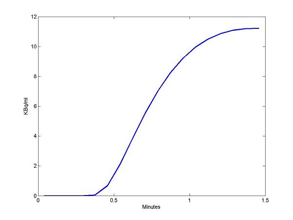
The above figure is the model output (CT). Here, we use it as perfect experimental data that would be fitted.
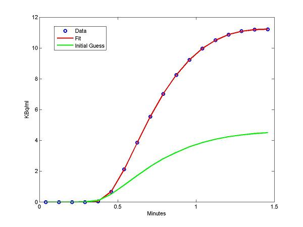
Step 3 Use model output as measured CT (perfect "data") and fit it
% Set parameters: initial guess, lower and upper bounds for K1, k2 and tau
pinit=[0.1;0.2;0.1];
lb   =[0.01;0.01;0.01];
ub   =[1;1;5];

% specify parameters to be adjusted in fitting
cm=addSensitivity(cm,'k1','k2','tau');

% Experimental Data to be fit
cm=set(cm,'ExperimentalData',sol(:,3));

% Perform curve fitting
[pfit,qfitnull,modelfit,pp1,output]=fitGen(cm,pinit,lb,ub,'OLS');
Step 4 Examine model outputs using estimated parameter (pfit) and initial guess (pinit)
% Solve model using estimated parameters
cm1=cm;
cm1=set(cm1,'ParameterValue','k1',pfit(1));
cm1=set(cm1,'ParameterValue','k2',pfit(2));
cm1=set(cm1,'ParameterValue','tau',pfit(3));
est_sol=solve(cm1);

% solve model using initial parameters
cm1=set(cm1,'ParameterValue','k1',pinit(1));
cm1=set(cm1,'ParameterValue','k2',pinit(2));
cm1=set(cm1,'ParameterValue','tau',pinit(3));
est_sol_init=solve(cm1);

plot(midScanTime,sol(:,3),'o',midScanTime,est_sol(:,3),'r-',midScanTime,est_sol_init(:,3),'g-','LineWidth',2);
xlabel('Minutes');
ylabel('KBq/ml');
legend('Data', 'Fit','Initial Guess');


