Support:Documents:Manual:COMKAT Command Line Interface
COMKAT Overview
Summary
COMKAT allows a user to construct a compartment model of his/her own design without resorting to writing equations. Models may then be used for a simulation and fitting data. COMKAT uses an object-oriented representation of models which is illustrated in this article.
Background
COMKAT enables a user to specify a model configuration without having to resort to writing and programming differential equations. This is all handled behind the scenes using state-of-the art differential equations solvers. On several platforms a solver written in C is used and transparently accessed from MATLAB via a mexfile interface created by the COMKAT authors. This means that solving the equations will be efficient and reliable. On platforms for which the compiled solver is not available, COMKAT will automatically use a differential equation solver (e.g. ode15s) from the MATLAB ODE Suite. This too will be reliable but may take more computer time.
Interfaces
There are two interfaces to COMKAT: a graphical user interface (GUI) and the command line interface (CLI). While the GUI has snazzy appeal and easy of use, the CLI is of particular utility to people doing modeling research. This is because the CLI enables one to set up simulations that loop and create thousands of simulated data sets. Because this is all done within the MATLAB environment, results of such simulations may be analyzed, graphed, and otherwise be prepared for publication. Alternatively, results could be saved to EXCEL spreadsheet or pasted into documents.
Principles
Modeling generally entails analyzing experimental data using mathematical rules that predict relationships between input functions, tissue responses and physiologic parameters. Modeling is used in two forms: 1 simulation or prediction and 2 fitting or characterization of function. In practice, to do fitting entails repeating simulations and adjusting values of parameters until the model-predicted output matches measured data. Consequently, 2 can be thought of as a superset of 1.
CompartmentModel Object
COMKAT uses an object-oriented approach to represent models. A compartmentModel object object can be thought of as the type for a variable that holds all the information needed to describe the kinetics, to setup and solve the equations, and even to fit data. Special functions called methods are used to configure the model, perform the solving and do the fitting. What makes something a method and not just a function is that a method acts on information stored in an object. While this might sound abstract and obtuse, hopefully the following example will convince you that this is a convenient, intuitive approach.
compartmentModel Object
Using the MATLAB command line interface (CLI), type this to create a new model object:
cm = compartmentModel;
Next use the whos command to see what was created:
>> whos cm
Name Size Bytes Class
cm     1x1 18830 compartmentModel object
Grand total is 428 elements using 18830 bytes
Notice that cm is not a double array, not an integer array and not even a structure. cm is a special data type created using the special function compartmentModel. This function is called a constructor because it creates new instance of an object. Actually, the function is a method. It is the constructor method for a compartmentModel object. (MATLAB "knows" that is a constructor since the name of the method, compartmentModel is the same as the name of the object type.)
At this point cm is a model with no compartments, no links connecting compartments, no data... as is revealed when examining its contents
>> cm
untitled1
Inputs: Name Spec. Act. Decay Const.
Compartments: Name (Saturation)
Outputs
Sensitivities
Links
Parameters: Name=Value
Note that nothing is special about the variable name cm. One could have just as easily created a compartmentModel object and called it Fred (Fred = compartmentModel;).
Compartments
Not much can be demonstrated with an empty model so we might as well create something useful. We start by adding a couple of compartments. Lets create a model that describes a hypothetical model of blood flow to the brain. The model will have two compartments one representing the brain and one representing the rest of the body.
>> brainModel = compartmentModel; % create a new, empty model
>> brainModel = addCompartment(brainModel, 'Brain');
>> brainModel = addCompartment(brainModel, 'Body');
[For those not familiar with MATLAB, % create a new, empty model is a comment. It is something that MATLAB ignores and is only for the convenience of the person reading the commands.]
Inputs
Lets assume that we are doing an imaging experiment and that something like radioactive water or gadolinium is administered intravenously to the subject. Blood in the carotid arteries will carry the material to the brain. Hence we consider the carotids as input function. That is, the time-course of the concentration of such a material in the blood would be experimentally measured. For the sake of simplicity lets assume that a MATLAB function called fengInput is created which can provide the blood concentration at time t. [In a more experimentally realistic case the concentration of the input function at time t may be determined by interpolating (e.g. linear interpolation) measured data. This can be done too and is, for the sake of keeping the present example simple, shown elsewhere.]
fengInput.m calculates the blood concentration at time t as a sum of gamma variate and exponential terms. The amplitudes and the exponential constants are all specified in input p to fengInput. For the sake of example, let p be defined as
>> p=[2 0 851.1 21.88 20.81 -4.134 -0.1191 -0.01043];
[The details of what each element of p means is not important to the current discussion.]
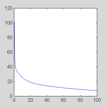
The following commands plot the input function concentration vs time [0., 0.1; 0.2, .... 100.0] minutes
>> p=[2 .5 16000 2188 2081 -7.5 -10 -0.01043];
>> t = [0:0.1:100];
>> plot(t,fengInput(p,t))
To include this input function in the model, use this command
>> brainModel = addInput(brainModel, 'Carotid', 1, 0, 'fengInput', p);
[For now don't worry about the 1 and 0 in the command. These are the specific activity (e.g. Bq/pmol) and tracer halflife (e.g. minutes). Because of the values used in this example the model can be interpreted as using a non-radioactive tracer or a tracer with infinite half life.]
Links
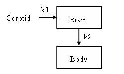
At this point the model has two compartments and one input but there is no specification as how tracer moves between the input and compartments. Herein we assume compartments are connected as depicted in the figure
To create the k1 link from the corotid input as the source to the brain as the destination, use this command
>> brainModel = addLink(brainModel, 'L', 'Carotid', 'Brain', 'k1');
[COMKAT is case-sensitive. Since the input was called Carotid in addInput(), it must be called Carotid in addLink() and not carotid and not CaRoTiD... You may use whatever mixture of upper and lower case that you prefer so long as you are consistent!]
The parameter 'L' in the statement identifies the link type. 'L' means the link source is an input and the kinetics are linear. To include the k2 link in the model the same type of command is used except that the linktype is 'K' because the link source is a compartment and not an input. [A list of the possible link types is given in the help for addLink.]
>> brainModel = addLink(brainModel, 'K', 'Brain', 'Body', 'k2');
For the mathematically inclined readers, we have just set up a model described by these equations:
 dBrain/dt = k1 • Corotid – k2 • Brain
 dBody/dt = k2 • Brain
Parameters
The next step is to assign values for the rate constants k1 and k2. These can be adjusted later so the values used here are not so critical. For now just assign k1 = 0.8, k2 = 0.5.
>> brainModel=addParameter(brainModel, 'k1', 0.8);
>> brainModel=addParameter(brainModel, 'k2', 0.5);
Model Output
At this point we are almost at the point where the model equations can be solved. What is missing is a specification of what is the model output. The output is not restricted to being the concentration in a single compartment but rather can be a weighted sum of the concentration in more than one compartment. Also there is the issue of defining the times at which solutions to the equations are desired. Model outputs are often defined as corresponding to the measured data. For example, pixel values may correspond to brain concentration averaged over the duration of the image acquisition.
Ignoring this time-averaging for a moment, an output might be thought of as one times the brain compartment concentration plus zero times the body compartment concentration. In COMKAT only the non-zero contributions of a compartment to outputs need be specified. Here is an example of how it might be done.
>> wlist = {'Brain', 1};
>> xlist = {};
>> brainModel=addOutput(brainModel, 'pixels', wlist, xlist);
The wlist defines the compartments and weights with which they contribut to outputs. (E.g. to define an output as 0.5*Brain + 0.4*Body, wlist = {'Brain', 0.5; 'Body', 0.4 }; xlist is similar to wlist except that xlist defines how input functions contribute directly to outputs. If for example, one would like the model the pixel as having 4% contribution from vascular space, do this xlist = {'Carotid', 0.04 };.)
To account for time-averaging inherent in data collection processes, we need only specify the the start and stop time of each image in the dynamic sequence. Lets assume the are 14 images and the start time (column 1) and end times (column 2 ) of each image is given in a MATLAB variable
>> st = [...
0    0.5
0.5  1
1    2
2    3
3    4
4    5
5   10
10  15
15  20
20  25
25  30
30  40
40  50
50  60
];
For example, image 3 (row 3 in st) begins at 1 minutes and ends at 2 minutes. To tell specify this in the model description, use the following command
>> brainModel = set(brainModel, 'ScanTime', st);
Solving the Model
At this point the model is completely defined and can be solved to obtain model-predicted concentration curves using the solve method:
>> [result, resultIndex] = solve(brainModel);
That is all there is to it. To see what we got, use the whos command
>> whos result
Name Size  Bytes Class
result 14x3 336    double array
The array result has as many rows as there images in the dyanmic image sequence. In this simple case the first column holds the scan start times, the second holds the scan end times and the third holds the output which was called 'pixels'. The number of columns and their contents depends on the model specification and all of this is described resultIndex
>> resultIndex
resultIndex =
'Scan Start'
'Scan End'
'pixels'
In general resultIndex{i} tells what is in column i of result.
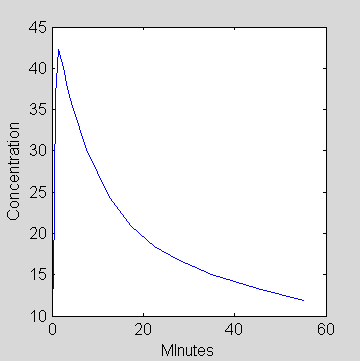
Standard MATLAB commands may be used to plot the pixel concentration versus the mid-time of each scan.
>> t=0.5*(result(:,1)+result(:,2)); % t is the mid-scan time
>> plot(t,result(:,3));
>> xlabel('MInutes')
>> ylabel('Concentration')
Closing Remarks
COMKAT allows a great deal of flexibility in defining, solving models and fitting models to data. This article just scratches the surface of the possiblities. This article focused on the command line interface (CLI) of COMKAT. Another article provides an introduction to the graphical user interface (GUI). Importantly, the GUI is just a "front end" that – behind the scenes – uses CLI.
COMKAT Command Line Function Reference
Command |
Syntax |
Comment |
|---|---|---|
| compartmentModel | cm = compartmentModel; | Creates a new compartment model object |
| addCompartment | cm2 = addCompartment(cm1, compartmentName[ ,saturationParameter]) | Adds a compartment to a model |
| addLink | cm2 = addLink(cm1, linkType, linkSource, linkDestination, linkName) | Adds a connection between two compartments or an input and a compartment |
| addInput | cm2 = addInput(cm1, inputName, specificActivity, decayConstant, functionName, inputParameter [, extraParameter]) | Adds an input to a model |
| addOutput | cm2 = addOutput(cm1, outputName, wSpec, xSpec) | Adds an output to a model (multiple outputs are supported) |
| addParameter | cm2 = addParameter(cm1, parameterName, parameterValue[, parameterMin, parameterMax]) | Adds a parameter to a model and specified initial value and optional limits on range |
| addSensitivity | cm2 = addSensitivity(cm1, parameterName) | Tells COMKAT that sensitivty functions are to be solved for the specified parameter(s). These parameters will be adjusted when fitting. |
| analyzeFit | [standardDeviation, covariance, correlation] = analyzeFit(cm1, jacobian, parameterFitValues, residuals) | Estimates precision of parameter estimates |
| cIdx | index = cIdx(cm1, compartmentName) | Returns compartment number associated with named compartment |
| dependsOn | yesNo = dependsOn(cm1, parmeter1, parameter2) | Returns 1 of parameter1 depends on parameter 2, 0 otherwise. parameter1 may be cell string array |
| exportAsScript | status = exportAsScript(cm1, fileName, variableName) | Creates a new file that contains COMKAT commands for creating the model in cm1. In the commands the model is put into the specified variable name. |
| fit | [newParmVal,modelfit,resnorm,residual,exitFlag,output,lambda,jacobian] = fit(cm, initParmVal, lb, ub) | Fit model to data returning parameter estimates and other optional information |
| fitGen |
[pfit, qfit, modelfit, exitflag, output, lambda, grad, hessian] = fitGen(cm, pinit, plb, pub) | Generalized fitting. Supports a number of different objective functions. |
| get | value = (cm1, property) | Retrieve information from compartment model object |
| getInputType | inputType = getInputType(cm, inputName) | Returns information about whether named input is used as a plasma concentration or as whole blood activity input |
| iIdx | index = iIdx(cm, inputName) | Retuns index number of named input. |
| load | cm2 = load(cm1, fileName) | Loads into memory a compartment model object that is stored in the specified mat file |
| pDeriv | dp1dp2 =pDeriv(cm, p1, p2) | Evaluates the partial derivative of parameter p1 with respect to parameter p2 |
| removeCompartment | cm2 = removeCompartment(cm1, idx) | Makes a copy of a model with compartment (specified by index) deleted |
| removeInput | cm2 = removeInput(cm1, input) | Returns a copy of the model with input deleted. Input may be specified by name or index |
| removeLink | cm2 = removeLink(cm1, idx) | Returns a copy of the model with link deleted. Link may be specified by name or index |
| save | cm2 = save(cm1, fileName) | Save specified compartment model object to the named mat file |
| set | cm2 = set(cm1, property, value[, one or more optional inputs]) | Set value of specified model property |
| solve | [PET, PETindex, component, componentIndex] = solve(cm) | Solve model equations |
Model construction basics
Summary
COMKAT allows a user to construct a model of his/her own design without resorting to writing equations.
Background
COMKAT enables a user to specify a model configuration without having to resort to writing and solving differential equations. This is all handled behind the scenes using state-of-the art differential equations solvers. On several platforms, the solver is written in C and accessed from MATLAB via a mexfile interface. This means that solving the equations will be efficient and reliable.
There are two interfaces to COMKAT: a graphical user interface (GUI) and the command line interface (CLI). While the GUI has snazzy appeal and easy of use, the CLI is the workhorse for people doing modeling research. This is because the CLI enables one to setup simulations that loop and create thousands of simulated data sets all within the MATLAB programming environment.
Principles
Modeling generally entails analyzing experimental data using mathematical rules that predict relationships between input functions, tissue responses and physiologic parameters. Values of physiologic parameters, such as perfusion, are estimated by adjusting their values until the model-predicted output agrees with the experimental data. Input function fitting is no different. One proposes a mathematical form as describing the input and then adjusts values of its parameters to achieve the best match between model-predicted and experimental data.
COMKAT Implementation
In this section an example is presented of using COMKAT to estimate parameters of the FDG input function. The first form of the example is intentionally kept simple to best illustrate concepts. The second example is more complex and perhaps a good starting point for you to research strategies for simultaneously estimating input functions and tissue kinetic parameters.
Example 1: Estimate Input Parameters, Rate Constants Known
Here we assume that the input function has the form
Cp = (p1t - p2 - p3) exp(-p4t) + p2 exp(-p5t) + p3 exp(-p6t)
where Cp is the plasma concentration of 18FDG, pi are the input function parameters to be estimated, and t is time. (This form comes from Feng, Huang, Wang. "Models for Computer simulation Studies of Input Functions for Tracer Kinetic Modeling with Positron Emission Tomography", International Journal of Biomedical Computing, 32(2):95-110, March 1993.)
Step 1 To set this up in MATLAB for simulation, create the following function and put it in a file called refCp.m:
function [fval, jac] = refCp(p, t)
 if (nargout > 0),
       t = t(:);  % make it a column vector
       fval = (p(1)*t - p(2) - p(3)) .* exp(-p(4)*t) + p(2) * exp(-p(5)*t) + p(3) * exp(-p(6)*t);
       if (nargout > 1),
           jac = [t .* exp(-p(4)*t) ...
                  -exp(-p(4)*t) + exp(-p(5)*t) ...
                  -exp(-p(4)*t) + exp(-p(6)*t) ...
                  -t .* (p(1)*t - p(2) - p(3)) .* exp(-p(4)*t) ...
                  -t * p(2) .* exp(-p(5)*t) ...
                  -t * p(3) .* exp(-p(6)*t)];
       end
   end
return
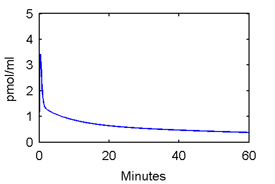
This function can be used to plot an example input curve using these commands
   t=0:.1:60;
   pin = [28 0.75 0.70 4.134 0.1191 0.01043];
   plot(t,refCp(pin,t))
   set(gca,'FontSize',6);
   axis([0 60 0 5]);
   xlabel('Minutes');
   ylabel('pmol/ml');
Note that he above function, refCp.m not only calculates values Cp, it also optionally calculates values for the derivative of Cp with respect to parameter vector p. These will be needed later since to fit the input function, it is important to quantify how changes in values of p will effects Cp values which, in turn, effect model-predicted tissue concentration reflected in voxels or regions of interest.
Step 2 Create an FDG model
   cm = compartmentModel;

   %        k1     k2      k3     k4
   ktrue=[0.1020 0.1300 0.0620 0.0068];

   % define the parameters
   cm = addParameter(cm, 'k1',    ktrue(1));     % 1/min
   cm = addParameter(cm, 'k2',    ktrue(2));     % 1/min
   cm = addParameter(cm, 'k3',    ktrue(3));     % ml/(pmol*min)
   cm = addParameter(cm, 'k4',    ktrue(4));     % 1/min
   cm = addParameter(cm, 'sa',    75);           % specific activity of injection, kBq/pmol
   cm = addParameter(cm, 'dk',    log(2)/109.8); % radioactive decay
   cm = addParameter(cm, 'PV',    1);            % (none)

   % define input function parameter vector
   cm = addParameter(cm, 'pin', [28; 0.75; 0.70; 4.134; 0.1191; 0.01043]);

   % define compartments
   cm = addCompartment(cm, 'Ce');
   cm = addCompartment(cm, 'Cm');
   cm = addCompartment(cm, 'Junk');

   % define plasma input function
   % specifying function as refCp with parameters pin
   cm = addInput(cm, 'Cp', 'sa', 'dk', 'refCp', 'pin'); % plamsa pmol/ml

   % connect inputs and compartments
   cm = addLink(cm, 'L', 'Cp', 'Ce', 'k1');
   cm = addLink(cm, 'K', 'Ce', 'Junk', 'k2');
   cm = addLink(cm, 'K', 'Ce', 'Cm', 'k3');
   cm = addLink(cm, 'K', 'Cm', 'Ce', 'k4');

   % specify scan begin and end times
   ttt=[ ones(6,1)*5/60; ...    %  6 frames x  5   sec
         ones(2,1)*15/60; ...   %  2 frames x 15   sec
         ones(6,1)*0.5;...      %  6 frames x  0.5 min
         ones(3,1)*2;...        %  3 frames x  2   min
         ones(2,1)*5;...        %  2 frames x  5   min
         ones(10,1)*10];        % 10 frames x 10   min
   scant = [[0;cumsum(ttt(1:(length(ttt)-1)))] cumsum(ttt)];
   cm = set(cm, 'ScanTime', scant);

   % define an output which is sum of Ce and Cm adjusted to account
   % for partial volume (PV).  Ignore vascular activity.
   Wlist = {...
       'Ce', 'PV';
       'Cm', 'PV'};
   Xlist = {};
   cm = addOutput(cm, 'PET', Wlist, Xlist);

   % solve model and generate example output
   [PET, PETindex]=solve(cm);
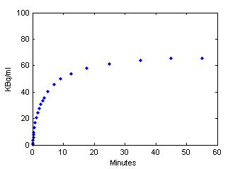
   plot(0.5*(PET(:,1)+PET(:,2)),PET(:,3), '.');
   set(gca,'FontSize',6);
   axis([0 60 0 100]);
   xlabel('Minutes');
   ylabel('KBq/ml');
Step 3 Use model output as perfect "data"
data = PET(:,3);
Step 4 Fit the "data"
   % tell model abbout data to be fit
   cm = set(cm, 'ExperimentalData', data);

   % specify parameters to be adjusted in fitting
   cm = addSensitivity(cm, 'pin');

   % set parameter values initial guess, lower and upper bounds
   pinit = [ 10; 0.4;  0.4;  3;  0.05; 0.01];
   plb =   [ 10; 0.1;  0.1;  1;  0.05; 0.001];
   pub =   [100; 2. ;  2. ; 10;  1.  ; 0.05];

   % actually do the fitting
   pfit = fit(cm, pinit, plb, pub);
Values of parameter pfit estimates are [28.0167; 0.7652; 0.7059; 4.1586; 0.1257; 0.0105] and are reasonably close to the true values (pxEval(cm, 'pin')) [28; 0.75; 0.70; 4.134; 0.1191; 0.01043]
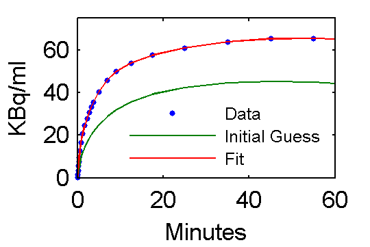
Step 5 Examine model outputs for "data", initial guess, and fit
   PETfit = solve(set(cm, 'ParameterValue', 'pin', pfit));
   PETinit = solve(set(cm, 'ParameterValue', 'pin', pinit));
   t = 0.5*(PET(:,1)+PET(:,2));
   plot(t,data,'.', t, PETinit(:,3), t, PETfit(:,3));
   set(gca,'FontSize',8);
   axis([0 60 0 75]);
   xlabel('Minutes');
   ylabel('KBq/ml');
   ah=legend('Data', 'Initial Guess', 'Fit','Location','SouthEast');
   set(ah,'FontSize',6,'Box','off');
Example 2: Simultaneously Estimate Input Parameters and Rate Constants
Aside from the obvious difference of estimatting values for rate constants as well as input parameters, this example simultaneoulsy fits three tissue regions. To do this, three different outputs (regA, regB, regC) are used and these are based on three different sets of compartments. We assume a single, common input.
Another important detail is that because of the way the K1 parameters appear in the differential equations - always multiplied by Cp, there is insufficient information to estimate both the K1 values and the scale of the input function. Think about it. It is what is called an identifiability problem. If you double K1 and halve Cp, their product - and hence model output - is unchange. Consequently, here we take the approach of fixing K1 values at their true value.
Step 1 Do nothing, just use the input from step 1 above.
Step 2 Create an FDG model for three regions all sharing the same input. (This example is a lot of typing or just one giant Copy and Paste. Nevertheless, it should be quite straightforward if you understood Example 1.
   cm = compartmentModel;  % start with a new, empty model

   %        k1     k2      k3     k4
   ktrueA=[0.1 ;  0.13 ; 0.06 ; 0.0068];
   ktrueB=[0.2 ;  0.25 ; 0.04 ; 0.0068];
   ktrueC=[0.05;  0.13 ; 0.02 ; 0.0068];

   % define the parameters
   cm = addParameter(cm, 'sa',    75);           % specific activity of injection, kBq/pmol
   cm = addParameter(cm, 'dk',    log(2)/109.8); % radioactive decay
   cm = addParameter(cm, 'PV',    1);            % (none)

   % region A
   cm = addParameter(cm, 'k1A',    ktrueA(1));     % 1/min
   cm = addParameter(cm, 'k2A',    ktrueA(2));     % 1/min
   cm = addParameter(cm, 'k3A',    ktrueA(3));     % ml/(pmol*min)
   cm = addParameter(cm, 'k4A',    ktrueA(4));     % 1/min

   % region B
   cm = addParameter(cm, 'k1B',    ktrueB(1));     % 1/min
   cm = addParameter(cm, 'k2B',    ktrueB(2));     % 1/min
   cm = addParameter(cm, 'k3B',    ktrueB(3));     % ml/(pmol*min)
   cm = addParameter(cm, 'k4B',    ktrueB(4));     % 1/min

   % region C
   cm = addParameter(cm, 'k1C',    ktrueC(1));     % 1/min
   cm = addParameter(cm, 'k2C',    ktrueC(2));     % 1/min
   cm = addParameter(cm, 'k3C',    ktrueC(3));     % ml/(pmol*min)
   cm = addParameter(cm, 'k4C',    ktrueC(4));     % 1/min

   % define input function parameter vector
   cm = addParameter(cm, 'pin', [28; 0.75; 0.70; 4.134; 0.1191; 0.01043]);

   % define compartments for regions A, B, C (they can share the same junk or sink compartment)
   cm = addCompartment(cm, 'Junk');
   cm = addCompartment(cm, 'CeA');
   cm = addCompartment(cm, 'CmA');
   cm = addCompartment(cm, 'CeB');
   cm = addCompartment(cm, 'CmB');
   cm = addCompartment(cm, 'CeC');
   cm = addCompartment(cm, 'CmC');

   % define plasma input function
   % specifying function as refCp with parameters pin
   cm = addInput(cm, 'Cp', 'sa', 'dk', 'refCp', 'pin'); % plamsa pmol/ml

   % connect inputs and compartments
   % region A
   cm = addLink(cm, 'L', 'Cp',  'CeA', 'k1A');
   cm = addLink(cm, 'K', 'CeA', 'Junk','k2A');
   cm = addLink(cm, 'K', 'CeA', 'CmA', 'k3A');
   cm = addLink(cm, 'K', 'CmA', 'CeA', 'k4A');

   % region B
   cm = addLink(cm, 'L', 'Cp',  'CeB', 'k1B');
   cm = addLink(cm, 'K', 'CeB', 'Junk','k2B');
   cm = addLink(cm, 'K', 'CeB', 'CmB', 'k3B');
   cm = addLink(cm, 'K', 'CmB', 'CeB', 'k4B');

   % region C
   cm = addLink(cm, 'L', 'Cp',  'CeC', 'k1C');
   cm = addLink(cm, 'K', 'CeC', 'Junk','k2C');
   cm = addLink(cm, 'K', 'CeC', 'CmC', 'k3C');
   cm = addLink(cm, 'K', 'CmC', 'CeC', 'k4C');

   % specify scan begin and end times
   ttt=[ ones(6,1)*5/60; ...    %  6 frames x  5   sec
         ones(2,1)*15/60; ...   %  2 frames x 15   sec
         ones(6,1)*0.5;...      %  6 frames x  0.5 min
         ones(3,1)*2;...        %  3 frames x  2   min
         ones(2,1)*5;...        %  2 frames x  5   min
         ones(10,1)*10];        % 10 frames x 10   min
   scant = [[0;cumsum(ttt(1:(length(ttt)-1)))] cumsum(ttt)];
   cm = set(cm, 'ScanTime', scant);
   % define an outputs, one for each region
   cm = addOutput(cm, 'RegA', {'CeA', 'PV'; 'CmA', 'PV'}, {});
   cm = addOutput(cm, 'RegB', {'CeB', 'PV'; 'CmB', 'PV'}, {});
   cm = addOutput(cm, 'RegC', {'CeC', 'PV'; 'CmC', 'PV'}, {});

   % solve model and generate example output
   [PET, PETindex]=solve(cm);
   idx = [3 4 5];
   plot(0.5*(PET(:,1)+PET(:,2)), PET(:,idx), '.');
   set(gca,'FontSize',6);
   xlabel('Minutes');
   ylabel('KBq/ml');
   axis([0 60 0 120]);
   ah=legend(PETindex(idx));
   set(ah,'FontSize',5,'Box','off');
Step 3 Use model output as perfect "data"
data = PET(:,idx); % data will have 3 columns, one for each region
Step 4 Fit the "data"
   % tell model abbout data to be fit
   cm = set(cm, 'ExperimentalData', data);

   % specify parameters to be adjusted in fitting
   cm = addSensitivity(cm, 'pin', 'k2A', 'k3A', 'k4A', 'k2B', 'k3B', 'k4B',  'k2C', 'k3C', 'k4C');

   % set parameter values initial guess, lower and upper bounds.  values are in same order as ensitivities
   %        _____________pin_________________  ______RegA______    ______RegB______  ______RegC______
   pinit = [ 10; 0.4;  0.4;  3;  0.05; 0.01;   0.1;  0.03; 0.001; 0.1;  0.03; 0.001; 0.1;  0.03; 0.001];
   plb =   [ 10; 0.1;  0.1;  1;  0.05; 0.001;  1e-3; 1e-3; 1e-3 ; 1e-3; 1e-3; 1e-3;  1e-3; 1e-3; 1e-3];
   pub =   [100; 2. ;  2. ; 10;  1.  ; 0.05;   1.;   1.;   1.;    1.;   1.;   1.;    1.;   1.;   1.];

   % actually do the fitting
   pfit = fit(cm, pinit, plb, pub);
Here are the results
         True       Fit
p1      28.0000  28.1555
p2      0.7500    0.9002
p3      0.7000    0.5201
p4      4.1340    4.1324
p5      0.1191    0.1240
p6      0.0104    0.0072
k2A    0.1300    0.1141
k3A    0.0600    0.0739
k4A    0.0068    0.0114
k2B    0.2500    0.2316
K3B    0.0400    0.0502
k4B    0.0068    0.0109
k2C    0.1300    0.1122
k3C    0.0200    0.0236
k4C    0.0068    0.0125
and, yes that is right, we just estimated values of 15 parameters. Wasn't that easy. Now lets see how well we did. Some or the parameters are estimated well; others are not.
Lets see how well well the curves fit the "data". For convenience, make a copy of the model setting the parameter to estimated values.
   cmfit = cm; % make a copy
   cmfit = set(cmfit, 'ParameterValue', 'pin', pfit(1:6));
   cmfit = set(cmfit, 'ParameterValue', 'k2A', pfit(7));
   cmfit = set(cmfit, 'ParameterValue', 'k3A', pfit(8));
   cmfit = set(cmfit, 'ParameterValue', 'k4A', pfit(9));
   cmfit = set(cmfit, 'ParameterValue', 'k2B', pfit(10));
   cmfit = set(cmfit, 'ParameterValue', 'k3B', pfit(11));
   cmfit = set(cmfit, 'ParameterValue', 'k4B', pfit(12));
   cmfit = set(cmfit, 'ParameterValue', 'k2C', pfit(13));
   cmfit = set(cmfit, 'ParameterValue', 'k3C', pfit(14));
   cmfit = set(cmfit, 'ParameterValue', 'k4C', pfit(15));
   set(gca,'FontSize', 6);
   PETfit = solve(cmfit);
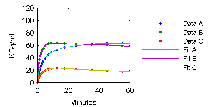
   plot(0.5*(PET(:,1)+PET(:,2)),PET(:,idx),'.',0.5*(PET(:,1)+PET(:,2)),PETfit(:,idx));
   axis([0 60 0 120]);
   ylabel('KBq/ml');
   xlabel('Minutes');
   ah=legend('Data A', 'Data B', 'Data C', 'Fit A', 'FIt B', 'Fit C','Location','EastOutside');
   set(ah,'FontSize',5,'Box','off');
The fits look pretty good so it appears the imperfect parameter estimates are a consequence of identifiability problems. This is described in another lesson.
